A unified theory for continuous in time evolving finite element space approximations to partial differential equations in evolving domains
Thomas Ranner
Preprint available arXiv:1703.04679. Slides available at tomranner.org/enumath2019

Motivation
Our aims
- Provide basic theory of how to construct and analyse finite element methods for parabolic problems in evolving domains
- This includes problems in evolving bulk domains, on evolving surfaces and coupled bulk-surface problems
- How to define and improve quality of moving meshes
- How to generalise (piecewise linear/isoparametric) surface finite elements to higher order elements
Model problem
Given “smoothly evolving smooth surface” \(\Gamma(t)\) find a scalar field \(u\) such that \[ \begin{align*} \partial^\bullet u + u \nabla_\Gamma \cdot w - \Delta_\Gamma u & = 0 \\ u(\cdot, 0) & = u_0. \end{align*} \]
(or general parabolic form on evolving surface, evolving domain, arbitrary parameterisations, …)
Recap on abstract theory of (Alphonse, Elliott, and Stinner 2015)
Compatibility
Let \(X(t)\) be a family of separable Hilbert spaces, \(\phi_t \colon X(0) \to X(t)\) homeomorphisms, the pair \((X(t), \phi_t)_{t \in [0,T]}\) are called compatible if \[ C_X^{-1} \| \phi_t \eta \|_{X(t)} \le \| \eta \|_{X(0)} \le C_X \| \phi_t \eta \|_{X(t)} \qquad \mbox{ for all } \eta \in X(0). \]
Consequences of compatibility
For a compatible pair \(( X(t), \phi_t )_{t \in [0,T]}\), we can define the Hilbert space \(L^2_X\): \[ \begin{multline*} L^2_\X := \Big\{ \eta \colon [0,T] \to \bigcup_{t \in [0,T]} \X(t) \times \{ t \}, t \mapsto ( \bar\eta(t), t ) : \\ \phi_{-\cdot} \bar\eta(\cdot) \in L^2( 0, T; \X_0 ) \Big\} \end{multline*} \] and strong material derivative \[ \md \eta := \phi_t \left( \dt (\phi_{-t} \eta) \right) \mbox{ for } \eta \in C^1_X. \]
Abstract formulation of the pde
Given an evolving Hilbert triple of compatible spaces \((V^*(t), H(t), V(t))\), find \(u \in L^2_V\) such that \[ m( t; \partial^\bullet u, \varphi ) + g( t; u, \varphi ) + a( t; u, \varphi ) = 0 \qquad \mbox{ for all } \varphi \in V(t). \]
Well posedness
Theorem. Under appropriate assumptions on the spaces, push-forward maps and bilinear forms, the continuous problem has a unique solution \(u\in L^2_V\) with \(\partial^\bullet u \in L^2_H\) which satisfies the stability bounds \[ \begin{align*} \sup_{t\in [0,T]} \| u \|_{H(t)}^2 + \int_0^T \| u \|_{V(t)}^2 \, d t & \le c(T) \| u_0 \|_{H_0}^2, \\ \sup_{t\in [0,T]} \| u \|_{V(t)}^2 + \int_0^T \| \partial^\bullet u \|_{H(t)}^2 \, d t & \le c(T) \| u_0 \|_{V_0}^2. \end{align*} \]
Evolving surface finite element spaces
Surface finite element reference map
Let \(( \hat{K}, \hat{P}, \hat{\Sigma} )\) be a reference finite element (i.e. standard) with \(\hat{K} \subset \R^n\). Let \(F_K\) satisfy:
• \(F_K \in C^1( \hat{K}, \R^{n+1} )\) • \(\text{rank} \nabla F_K = n\) • \(F_K\) is injective,
and that \(F_K\) can be decomposed into an affine and smooth part: \[ F_K( \hat{x} ) = A_K \hat{x} + b_k + D_K( \hat{x} ) \] such that \(A_K\) has full column rank, \(D_K \in C^1( \hat{K} )\) and \[ C_K := \sup_{\hat{x} \in \hat{K}} \norm{ \nabla D_K( \hat{x} ) A_K^\dagger } < 1. \] In this case, we call \(F_K\) a surface finite element reference map.
Surface finite element
Let \(( \hat{K}, \hat{P}, \hat{\Sigma} )\) be a reference finite element (i.e. standard) with \(\hat{K} \subset \R^n\), \(F_K\) a surface finite element reference map, and the triple \((K, P, \Sigma)\) given by
- \(K := F_K( \hat{K} )\) (the element domain)
- \(P := \{ \hat\chi \circ F_K^{-1} : \hat{\chi} \in \hat{P} \}\) (the shape functions)
- \(\Sigma := \{ \chi \mapsto \hat{\sigma}( \chi \circ F_K ) : \hat{\sigma} \in \hat\Sigma \}\) ( the nodal variables).
Then we call \((K, P, \Sigma)\) a surface finite element.
\(\Theta\)-surface finite element
If in addition
- \(F_K \in C^{\Theta+1}( \hat{K}; \R^{n+1} )\)
- for \(1 \le m \le \Theta+1\) \[ \sup_{\hat{x} \in \hat{K}} \abs{ \nabla^m F_K( \hat{x} ) } \norm{ A_K }^{-m} \le C_M( K ) \]
- \(P\) contains \(\hat{\chi} \circ F_K^{-1}\) for all \(\hat{\chi} \in P_\Theta( \hat{K} )\)
- \(P \subset C^{\Theta+1}( K )\)
then we call \((K, P, \Sigma)\) a \(\Theta\)-surface finite element.
see also (Bernardi 1989)
Examples

Norm scaling properties
If \(\chi \in W^{m,p}( K )\) then \(\hat\chi = \chi \circ F_K \in W^{m,p}(\hat{K})\) and \[ \abs{ \hat{\chi} }_{W^{m,p}( \hat{K} ) } \le c \meas(K)^{-1/p} \norm{ A_K }^m \sum_{r=1}^m \abs{ \chi }_{W^{r,p}(K)}. \] If \(\hat{\chi} \in W^{m,p}( \hat{K} )\) then \(\chi = \hat\chi \circ F_K^{-1} \in W^{m,p}( \hat{K} )\) and \[ \abs{ \chi }_{W^{m,p}( K )} \le c \meas(K)^{1/p} \sum_{r=1}^m \norm{ A_K^\dagger }^r \norm{ \hat\chi }_{W^{r,p}( \hat{K} ) }. \]
Interpolation property
If the reference element satisfies a Bramble-Hilbert Lemma then for all \(\chi \in W^{k+1,p}( K )\) \[ \abs{ \chi - I_K \chi }_{W^{m,p}(K)} \le c\, \text{meas}(K)^{1/q - 1/p} \frac{h_K^{k+1}}{\rho_K^m} \abs{ \chi }_{W^{k+1,p}(K)}. \]
How to bring several elements together?
We restrict to Lagrange finite elements: \[ \Sigma := \{ \chi \mapsto \chi( a ) : a \in N^K \}. \]
Let \(\Gamma_h\) be discrete surface with conforming subdivision \(\T_h\). We assume that for any two adjacent (i.e. which share a common facet) surface finite elements \((K, P, \Sigma)\) and \((K', P', \Sigma' )\) that \[ \left( \bigcup_{a \in N^K} a \right) \cap K' = \left( \bigcup_{a' \in N^{K'}} a' \right) \cap K. \]
Surface finite element space
Let each \(K \in \T_h\) have an associated surface finite element \((K, P^K, \Sigma^K)\). A surface finite element space is a (proper) subset of the product space \(\prod P^K\) given by \[ \begin{multline*} \S_h := \Big\{ \chi_h = ( \chi_K )_{K \in \T_h} \in \prod_{K \in \T_h} P^K : \\ \chi_K( a ) = \chi_{K'}( a ) \text{ for all } K, K' \in \T( a ), \text{ and all } a \in N_h \Big\}. \end{multline*} \]
Lemma. We can identify each \(\chi_h \in \S_h\) with a continuous function.
Examples
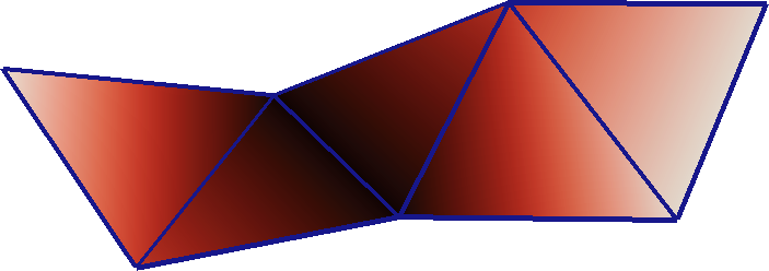
Piecewise linear function
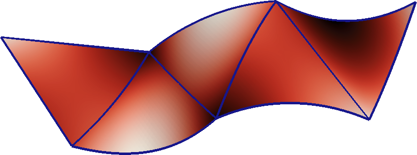
Piecewise quadratic function
Evolving surface finite element
We say the family \((K(t), P(t), \Sigma(t))_{t \in [0,T]}\) is a evolving surface finite element if
- each share a common reference element
- \[ C_K := \sup_{t \in [0,T]} \sup_{\hat{x} \in \hat{K}} \norm{ D \Phi( \hat{x}, t ) A_K^\dagger(t) } < c < 1. \]
We say the family \((K(t), P(t), \Sigma(t))_{t \in [0,T]}\) is a \(\Theta\)-evolving surface finite element if
- each \(( K(t), P(t), \Sigma(t) )\) is a \(\Theta\)-surface finite element
- \[ \sup_{t \in [0,T]} C_m( K(t) ) \le c \le \infty \qquad \text{ for } 1 \le m \le \Theta+1. \]
Element flow map
There exists a family of maps \(\Phi^K_t \colon K_0 \to K(t)\) called the flow map given by \[ F_{K(t)} ( \hat{x} ) = \Phi^K_t( F_{K_0}( \hat{x} ) ). \]
The flow map defines the element velocity field by \[ W_K( \Phi^K_t(x), t ) = \dt \Phi^K_t( x ). \]
Element push forward map
The family of element push forward maps \(\phi^K_t\) is defined for \(\chi \colon K_0 \to \R\) by \(\phi^K_t \chi \colon K(t) \to \R\) where \[ \phi^K_t( \chi )( x ) = \chi( \Phi^K_{-t}( x ) ). \]
Compatibility
We say that \((K(t), P(t), \Sigma(t))_{t \in [0,T]}\) is temporally quasi-uniform if there exists \(\rho_K > 0\) such that \[ \inf \{ \rho_{K(t)} : t \in [0,T] \} \ge \rho_K h. \]
Lemma. If an \(\Theta\)-evolving surface finite element \((K(t), P(t), \Sigma(t))_{t \in [0,T]}\) is temporally quasi-uniform then \(( W^{m,p}(K(t)), \phi^K_t)_{t \in [0,T]}\) (for \(0 \le m \le \Theta\), \(p \in [1,\infty]\)) and \(( P(t), \phi^K_t )_{t \in [0,T]}\) form compatible pairs.
Evolving surface finite element space
We restrict that element flow maps coincide at Lagrange points: for all \(a_0 \in N_h(0)\) we have \[ \Phi^K_t( a_0 ) = \Phi^{K'}_t( a_0 ) \text{ for adjacent } K(t), K'(t). \]
An evolving surface finite element space \(\S_h(t)\) is a time-dependent family of surface finite element spaces consisting of evolving surface finite elements.
Compatibility
We define a global push forward map for \(\eta_h \colon \Gamma_{h,0} \to \R\) by \(\phi^h_t \eta_h \colon \Gamma_h(t) \to \R\) by \[ ( \phi^h_t \eta_h )|_{K(t)} = \eta_h \circ \Phi^K_{-t}. \]
Lemma. If \(\T_h(t)\) is a uniformly quasi-uniform subdivision then each element is temporally quasi-uniform. In particular \(( W^{m,p}( \T_h(t), \phi^h_t ) )_{t \in [0,T]}\) (for \(0 \le m \le \Theta+1\), \(p \in [1,\infty]\)) and \(( \S_h(t), \phi^h_t )_{t \in [0,T]}\) are compatible pairs.
Material derivatives
Let \(H_h( t ) := L^2( \T_h(t) )\). We have that \((L^2( \T_h(t)), \phi^K_t)_{t \in [0,T]}\) form a compatible pair
- we can define the spaces \(L^2_{H_h}\) and \(C^1_{H_h}\)
- we can define a discrete material derivative \[ \md_h \eta_h := \phi_t^h \left( \dt \phi^h_{-t} \eta_h \right). \]
Lemma. Denote by \(\{ \chi_j( \cdot, t )\}_{j=1}^N\) the set of global basis functions. Then \(\md_h \chi_j = 0\).
Relation to continuous problem
We don’t have time in this talk to go into details….
Relating these definitions to their continuous counterparts requires lifting operators:
- \(\Lambda_K \colon K(t) \to \Gamma\)
- \(\lambda_h \colon H_h(t) \to H(t)\).
This also provides an interpolation operator \(I_h \colon C( \Gamma ) \to \S_h^\ell\).
Application
Construction of initial discrete surface

At initial time use interpolation of normal projection operator to define initial surface finite element reference map. Examples shown for isoparametric elements \(k=1,2,3\).
Construction of evolving discrete surface

Construct discrete flow map as interpolation of smooth flow map: Lagrange points move with velocity \(w\).
Evolving surface finite element space
Let \(\S_h(t)\) be an isoparametric finite element space over \(\T_h(t)\) (Demlow 2009; Kovács 2018). Assume that the evolving subdivision \(\{ \T_h(t) \}_{t \in [0,T]}\) is uniformly quasi-uniform.
Proposition. The above construction defines \(\S_h(t)\) to be an evolving surface finite element space consisting of \(k\)-evolving surface finite elements and the corresponding pair \(( \S_h(t), \phi^h_t )_{t \in [0,T]}\) form a compatible pair.
Further analysis of finite element scheme
- We also give details of stability and error analyses based on an abstract formulation.
- The results give show quasi-optimal error bounds for a general parabolic problem on an evolving open domain, evolving surface and a coupled bulk surface problem.
- I do not have time to give any further details…
Numerical results
Consider \(\Gamma_0 = S^2 \subset \R^3\) the unit sphere and define \(\Gamma(t)\) by the velocity: \[ w( x, t ) = \left( \frac{\cos(t) x_1}{8(1+1/4 \sin(t))}, 0, 0 \right). \] For solution we take \(u(x,t) = \sin(t) x_2 x_3\) and consider a general parabolic operator with \(\A = ( 1 + x_1^2 ) \id\), \(\B = ( 1,2,0) - ( 1,2,0) \cdot \nu \nu\), \(\C = \sin(x_1 x_2)\)
Choose \(k=3\), time step to recover optimal scaling.
Numerical results
| \(h\) | \(\tau\) | \(L^2(\Gamma(T))\) error | (eoc) |
|---|---|---|---|
| \(8.31246\cdot10^{-1}\) | \(1.00000\) | \(9.88086\cdot10^{-2}\) | — |
| \(4.40053\cdot10^{-1}\) | \(6.25000\cdot10^{-2}\) | \(7.60635\cdot10^{-3}\) | \(4.03157\) |
| \(2.22895\cdot10^{-1}\) | \(3.90625\cdot10^{-3}\) | \(4.92316\cdot10^{-4}\) | \(4.02476\) |
| \(1.11969\cdot10^{-1}\) | \(2.44141\cdot10^{-4}\) | \(3.08257\cdot10^{-5}\) | \(4.02448\) |
| \(5.60891\cdot10^{-2}\) | \(1.52588\cdot10^{-5}\) | \(1.89574\cdot10^{-6}\) | \(4.03416\) |
Summary
- We have shown fundamental definitions of an evolving surface finite element space
- We have (briefly) considered one particular realisation using isoparametric surface finite elements
- We have given ideas of how one might generalise this theory
- We have not shown how this relates to an abstract finite element analysis to show stability and error bounds
- We have not shown similar constructions for problems in evolving bulk domains
Thank you for your attention! Preprint available arXiv:1703.04679. Slides available at tomranner.org/enumath2019
References
Alphonse, A., C. M. Elliott, and B. Stinner. 2015. “An Abstract Framework for Parabolic PDEs on Evolving Spaces.” Port. Math. 72 (1): 1–46. https://doi.org/10.4171/PM/1955.
Bernardi, C. 1989. “Optimal Finite-Element Interpolation on Curved Domains.” SIAM Journal on Numerical Analysis 26 (5). SIAM: 1212–40. https://doi.org/10.1137/0726068.
Demlow, A. 2009. “Higher-order finite element methods and pointwise error estimates for elliptic problems on surface.” SIAM Journal on Numerical Analysis 47 (2): 805–27. https://doi.org/10.1137/070708135.
Dziuk, G. 1988. “Finite Elements for the Beltrami operator on arbitrary surfaces.” In Partial Differential Equations and Calculus of Variations, edited by Stefan Hildebrandt and Rolf Leis, 1357:142–55. Lecture Notes in Mathematics. Berlin: Springer-Verlag. https://doi.org/10.1007/BFb0082865.
Heine, C. J. 2005. “Isoparametric finite element approximation of curvature on hypersurfaces.” Freiburg. http://citeseerx.ist.psu.edu/viewdoc/download?doi=10.1.1.574.7294&rep=rep1&type=pdf.
Kovács, B. 2018. “High-Order Evolving Surface Finite Element Method for Parabolic Problems on Evolving Surfaces.” IMA Journal of Numerical Analysis 38: 430–59. https://doi.org/10.1093/imanum/drx013.
Vierling, M. 2014. “Parabolic optimal control problems on evolving surfaces subject to point-wise box constraints on the control – theory and numerical realization.” Interfaces and Free Boundaries 16 (2): 137–73. https://doi.org/10.4171/IFB/316.