A stable finite element method for an open, inextensible, viscoelastic rod with applications to nematode locomotion
Tom Ranner
Slides available at tomranner.org/interfaces2021 | Paper doi:10.1016/j.apnum.2020.05.009

Motivation
C. elegans locomotion in three dimensions
- 1mm long
- 40 μm wide (~hair width)
- Move by passing a travelling wave of muscle contractions down body
- Muscle contractions generate bending (preferred curvature)
- Thrust is in opposite direction to thrust due to anisotropic drag from surrounding fluid (low Reynolds, gel)
The mechanical model
The muscles
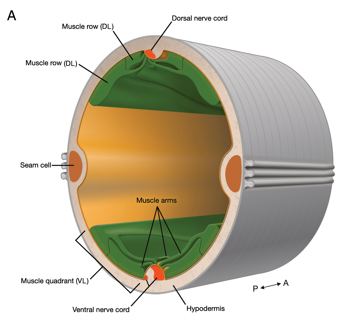
doi:10.3908/wormatlas.1.7 | From Omer Yuval
Framed curve: Kirchhoff-Love rod
Frame equations
Any (smooth) frame \((\vec{\tau}, \vec{e}_1, \vec{e}_2)\) defines three scalar fields \(\alpha, \beta\) and \(\gamma\) which satisfy:
\[ \frac{1}{|\vec{x}_u|} \vec{\tau}_u = \alpha \vec{e}^1 + \beta \vec{e}^2, \\ \frac{1}{|\vec{x}_u|} \vec{e}^1_u = -\alpha \vec{\tau} + \gamma \vec{e}^2, \\ \frac{1}{|\vec{x}_u|} \vec{e}^2_u = -\beta \tau - \gamma \vec{e}^1. \]
This corresponds to (vector) curvature \(\vec{\kappa} = \alpha \vec{e}^1 + \beta \vec{e}^2\) and twist \(\gamma\).
We also define angular moment similarly: \(\vec\omega = \vec\tau \times \vec\tau_t + m \vec \tau\) so that \[ \partial_t \vec{e}_1 = - \vec{e}_1 \cdot \vec{\tau}_t \vec\tau + m \vec{\tau}, \partial_t \vec{e}_2 = - \vec{e}_2 \cdot \vec{\tau}_t \vec\tau - m \vec{\tau}. \]
Model ingredients
- Total moment \[\vec{M} = \vec{\tau} \times \vec{y} + z \vec{\tau},\]
- Bending moment \[\vec{y} = A ((\alpha-\alpha^0) \vec{e}_1 + (\beta - \beta^0) \vec{e}_2) + B (\alpha_t \vec{e}_1 + \beta_t \vec{e}_2).\]
- Twisting moment \[z = C (\gamma - \gamma^0) + D \gamma_t.\]
- Environment forces: (resistive forces, not fundamental derivation) \[ \vec{D}_{\text{lin}} = K_\tau (\vec\tau \otimes \vec\tau) \vec{x}_t + K_\nu ( {\mathbb{I}}- \vec\tau \otimes \vec\tau ) \vec{x}_t, \qquad \vec{D}_\text{rot} = -K_\text{rot} m \vec{\tau} \]
Summary of equations and unknowns
Unknowns
- \(\vec{x}\) - position
- \(p\) - line tension
- \(\vec{\kappa}\) - vector curvature
- \(\gamma\) - twist
- \(\vec{y}\) - bending moment
- \(z\) - twisting moment
- \(m\) - tangential angular momentum
- \(\vec{e}_1, \vec{e}_2\) - the frame
Equations
- Two from balance laws
- Two from geometry
- Two from moment constitutive laws
- Inextensibility constraint
- Frame update equations
- Boundary and initial conditions
Equations look like fourth order parabolic equation for \(x\), with local length constraint, coupled to second order parabolic equation for anti-derivative of \(\gamma\).
Discretization
Discretization ideas
We split the domain \((0,1)\) into equal elements of length \(h\) and choose a time step \(\Delta t\)
We use a combination of piecewise linear finite elements \(V_h\) and piecewise constant functions \(Q_h\).
Use mass lumping for vertex-wise updates.
Two tangent vectors
For a discrete parametrisation \(\vec{x}_h \in V_h^3\), we introduce two different tangent vector fields.
\(\vec{\tau}_h \in Q_h^3\) as the piecewise constant normalised derivative of \(\vec{x}_h\): \(\vec{\tau}_h = {\vec{x}_{h,u}} / { |\vec{x}_{h,u}| }\).
\(\tilde{\vec{\tau}}_h \in V_h^3\) with vertex values given by \[ \tilde{\vec{\tau}}_h( u_j, \cdot ) = \frac{ \vec{\tau}_{h}( u_i^-, \cdot) + \vec{\tau}_h( u_i^+, \cdot ) }{| \vec{\tau}_{h}( u_i^-, \cdot) + \vec{\tau}_h( u_i^+, \cdot ) |} \quad \mbox{ for } i = 1, \ldots, N, \]
where \(\vec\tau_h( u_i^\pm, \cdot )\) is \(\vec{\tau}_h\) evaluated on the left (or right) element to the vertex \(u_i\).
Discretization choices
| Variable | Name | Discrete variable | Space |
|---|---|---|---|
| \(\vec{x}\) | position | \(\vec{x}_h\) | \(V_h^3\) |
| \(p\) | line tension | \(p_h\) | \(Q_h\) |
| \(\vec{\kappa}\) | vector curvature | \(\vec{\kappa}_h\) | \(V_h^3\) |
| \(\gamma\) | twist | \(\gamma_h\) | \(Q_h\) |
| \(\vec{y}\) | bending moment | \(\vec{y}_h\) | \(V_h^3\) |
| \(z\) | twisting moment | \(z_h\) | \(Q_h\) |
| \(m\) | tangential angular momentum | \(m_h\) | \(V_h\) |
| \(\vec{e}_1, \vec{e}_2\) | the frame | \(\vec{e}_{1,h}, \vec{e}_{2,h}\) | \(V_h^3\) |
Semi-discrete scheme
Given preferred curvatures \(\alpha^0, \beta^0\), a preferred twist \(\gamma_0\), and initial conditions for \(\vec{x}_h, \gamma_h\) (which imply compatible initial conditions for \(\vec{w}_h\), \(\vec{e}_{1,h}\) and \(\vec{e}_{2,h}\) up to a fixed rotation), for \(t \in [0,T]\), find \(\vec{x}_h( \cdot, t) \in V_h^3, \vec{y}_h( \cdot, t) \in V_{h,0}^3, \vec{w}_h( \cdot, t ) \in V_{h,0}^3 + \vec{w}_b(\cdot,t)\),\(m_h( \cdot, t ) \in V_h, z_h( \cdot, t ), \gamma_h( \cdot, t), p_h( \cdot, t ) \in Q_h\), \(\vec{e}_{h,1}( \cdot, t ), \vec{e}_{h,2}( \cdot, t ) \in V_h^3\) such that
\[ \begin{align} \label{eq:fem-x} \int_0^1 \K \vec{x}_{h,t} \cdot \vec{\phi}_h | \vec{x}_{h,u} | - \int_0^1 p_h \vec\tau_h \cdot \vec{\phi}_{h,u} \qquad\qquad\qquad\qquad\qquad\qquad & \\ \nonumber - \int_0^1 \bigl( ( \id - \vec\tau_h \otimes \vec\tau_h ) \frac{\vec{y}_{h,u}}{| \vec{x}_{h,u} |} + z_h \vec\tau_h \times \vec{w}_h \bigr) \cdot \vec{\phi}_{h,u} & = 0 \\ % \label{eq:fem-y} \int_0^1 \Bigl( \bigl( \vec{y}_h - A ( \vec{w}_h - \alpha^0 \vec{e}_{1,h} - \beta^0 \vec{e}_{2,h} ) \qquad\qquad\qquad\qquad\qquad\qquad & \\ \nonumber - B ( ( \id - \tilde{\vec\tau}_h \otimes \tilde{\vec\tau}_h ) \vec{w}_{h,t} - m_h \tilde{\vec\tau}_h \times \vec{w}_h ) \bigr) \cdot \vec{\psi}_h \Bigr)_h | \vec{x}_{h,u} | & = 0 \\ % \label{eq:fem-w} \int_0^1 ( \vec{w}_h \cdot \vec\psi_h )_h | \vec{x}_{h,u} | + \frac{\vec{x}_{h,u}}{ | \vec{x}_{h,u} | } \cdot \vec\psi_{h,u} & = 0 \end{align} \] for all \(\vec\phi_h \in V_h^3\), \(\vec\psi_h \in V_{h,0}^3\), \[ \begin{align} \label{eq:fem-gamma} \int_0^1 - ( K^\rot m_h v_h )_h | \vec{x}_{h,u} | - \int_0^1 z_h v_{h,u} + \int_0^1 ( \vec{y}_h \cdot ( \tilde{\vec\tau}_h \times \vec{w}_h ) v_h )_h | \vec{x}_{h,u} | & = 0, \\ % \label{eq:fem-z} \int_0^1 ( z_h - C ( \gamma_h - \gamma^0 ) - D \gamma_{h,t} ) q_h | \vec{x}_{h,u} | & = 0, \\ % \label{eq:fem-m} \int_0^1 \gamma_{h,t} q_h | \vec{x}_{h,u} | - \int_0^1 m_{u,h} q_h + \int_0^1 \vec\tau_h \times \vec{w}_h \cdot \vec{x}_{h,tu} q_h & = 0 \end{align} \] for all \(q_h \in Q_h\) and \(v_h \in V_h\), \[ \begin{align} \label{eq:fem-p} \int_0^1 q_h \vec\tau_h \cdot \vec{x}_{h,tu} & = 0, \end{align} \] for all \(q_h \in Q_h\), and \[ \begin{equation} \label{eq:fem-frame} \int_0^1 \Bigl( \bigl( \vec{e}_{h,j,t} - \bigl( \tilde{\vec{\tau}}_h \times \tilde{\vec{\tau}}_{h,t} + m_h \tilde{\vec{\tau}}_h \bigr) \times \vec{e}_{h,j} \bigr) \cdot \vec{\phi}_h \Bigr)_h | \vec{x}_{h,u} | = 0, \mbox{ for } j = 1,2, \end{equation} \] for all \(\vec{\phi}_h\in V_h^3\).
Semi-discrete stability
Lemma If \(\alpha^0, \beta^0, \gamma^0\) are independent of time, any solution to the above problem satisfies: \[ \begin{multline*} \int_0^1 ( \K \vec{x}_{h,t} \cdot \vec{x}_{h,t} + K^\rot m_h^2 ) | \vec{x}_{h,u} | \\ + \frac{1}{2} \ddt \int_0^1 \bigl( A \bigl( ( \alpha_h - \alpha^0 )^2 + ( \beta_h - \beta^0 )^2 \bigr)_h + C ( \gamma_h - \gamma^0 )^2 \bigr) | \vec{x}_{h,u} | \\ + \int_0^1 \bigl( ( B ( \alpha_{h,t}^2 + \beta_{h,t}^2 ) )_h + D \gamma_{h,t}^2 \bigr) | \vec{x}_{h,u} | = 0. \end{multline*} \]
Full discrete scheme
Given preferred curvatures \(\alpha^0, \beta^0\), a preferred twist \(\gamma^0\), and initial conditions for \(\vec{x}_h^0, \gamma_h^0\), (which imply compatible initial conditions for \(\vec{w}_h^0\), \(\vec{e}_{1,h}^0\), \(\vec{e}_{2,h}^0\) up to a fixed rotation), for \(n = 1, \ldots, M\) find \(\vec{x}_h^n \in V_h^3, \vec{y}_h^n \in V_{h,0}^3, \vec{w}_h^n \in V_{h,0}^3 + \vec{w}_{b}^n\), \(m_h^n \in V_h, z_h^n, \gamma_h^n, p_h^n \in Q_h\), \(\vec{e}_{h,1}^n, \vec{e}_{h,2}^n \in V_h^3\) such that \[ \begin{align} \label{eq:discrete-x} \int_0^1 \K \bar\partial \vec{x}_{h}^n \cdot \vec{\phi}_h | \vec{x}_{h,u}^{n-1} | - \int_0^1 p_h^n \vec\tau_h \cdot \vec{\phi}_{h,u} \qquad\qquad\qquad\qquad\qquad\qquad \\ \nonumber - \int_0^1 \bigl( ( \id - \vec\tau_h^{n-1} \otimes \vec\tau_h^{n-1} ) \frac{1}{| \vec{x}_{h,u}^{n-1} |} \vec{y}_{h,u}^n + z_h^n \vec\tau_h^{n-1} \times \vec{w}_h^{n-1} \bigr) \cdot \vec{\phi}_{h,u} & = 0 \\ % \label{eq:discrete-y} \int_0^1 \bigl( \vec{y}_h^{n} - A ( \vec{w}_h^n - \alpha^0( \cdot, t^n ) \vec{e}_{1,h}^{n-1} - \beta^0( \cdot, t^n ) \vec{e}_{2,h}^{n-1} ) \qquad\qquad\qquad\qquad \\ \nonumber - B \bigl( ( \id - \tilde{\vec\tau}_h^{n-1} \otimes \tilde{\vec\tau}_h^{n-1} ) \bar\partial \vec{w}_{h}^n - m_h^{n-1} \tilde{\vec\tau}_h^{n-1} \vec{w}_h^n \bigr)_h \bigr) \cdot \vec\psi_h | \vec{x}_{h,u}^{n-1} | & = 0 \\ \label{eq:discrete-w} \int_0^1 \vec{w}_h^{n} \cdot \vec\psi_h | \vec{x}_{h,u}^{n-1} | + \frac{1}{ | \vec{x}_{h,u}^{n-1} | } \vec{x}_{h,u}^n \cdot \vec\psi_{h,u} & = 0 \end{align} \] for all \(\vec\phi_h \in V_h^3\), \(\vec\psi_h \in V_{h,0}^3\), \[ \begin{align} \label{eq:discrete-gamma} \int_0^1 - K^\rot m_h^n v_h | \vec{x}_{h,u}^{n-1} | - \int_0^1 z_h^n v_{h,u} + \int_0^1 \vec{y}_h^{n-1} \cdot ( \tilde{\vec\tau}_h^{n-1} \times \vec{w}_h^{n-1} ) v_h | \vec{x}_{h,u}^{n-1} | & = 0, \\ % \label{eq:discrete-z} \int_0^1 ( z_h^n - C ( \gamma_h^n - \gamma^0( \cdot, t^n) ) - D \bar\partial \gamma_{h}^n ) q_h | \vec{x}_{h,u}^{n-1} | & = 0, \\ % \label{eq:discrete-m} \int_0^1 \bar\partial \gamma_{h}^n q_h | \vec{x}_{h,u}^{n-1} | - \int_0^1 m_{u,h} q_h + \int_0^1 ( \vec\tau_h^{n-1} \times \vec{w}_h^{n-1} ) \cdot \bar\partial \vec{x}_{h,u}^n q_h & = 0 \end{align} \] for all \(q_h \in Q_h\) and \(v_h \in V_h\), \[ \begin{align} \label{eq:discrete-p} \int_0^1 q_h \vec\tau_h^{n-1} \cdot \vec{x}_{h,u}^n & = \int_0^1 | \vec{x}_{h,0,u} | q_h, \end{align} \] for all \(q_h \in Q_h\). Using the abbreviations: \[ \begin{align} \vec{k}_i^n & = \tilde{\vec\tau}_h^{n-1}( u_i ) \times \tilde{\vec\tau}_h^n( u_i ), &\vec{l}_i^n & = \tilde{\vec{\tau}}^n_h( u_i ), & \varphi_i^n & = \Delta t \, m_h^n( u_i ), \end{align} \] we apply the Rodrigues formula twice: \[ \begin{align} \label{eq:discrete-e1-R1} \tilde{\vec{e}}_{j,h}^n( u_i ) & = \vec{e}_{j,h}^{n-1}( u_i ) ( \tilde{\vec\tau}_h^{n-1}( u_i ) \cdot \tilde{\vec\tau}_h^{n}( u_i )) + \vec{k}_i^n \times \vec{e}_{j,h}^{n-1}( u_i ) \\ \nonumber & \qquad + \vec{e}_{j,h}^{n-1}( u_i ) \cdot \vec{k}_i^n \vec{k}_i^n \frac{1}{1 + \tilde{\vec\tau}_h^{n-1}( u_i ) \cdot \tilde{\vec\tau}_h^{n}( u_i )} && j=1,2 \\ % \label{eq:discrete-e1-R2} {\vec{e}}_{j,h}^n( u_i ) & = \tilde{\vec{e}}_{j,h}^n( u_i ) \cos( \varphi_i ) + \vec{l}_i^n \times \tilde{\vec{e}}_{j,h}^n( u_i ) \sin( \varphi_i ) \\ \nonumber & \qquad + ( \tilde{\vec{e}}_{j,h}^n( u_i ) \cdot \vec{l}_i^n )\vec{l}_i^n ( 1 - \cos( \varphi_i ) ) && j=1,2. \end{align} \]
Full discrete scheme: frame update
Using the abbreviations: \[ \vec{k}_i^n = \tilde{\vec\tau}_h^{n-1}( u_i ) \times \tilde{\vec\tau}_h^n( u_i ), \vec{l}_i^n = \tilde{\vec{\tau}}^n_h( u_i ), \varphi_i^n = \Delta t \, m_h^n( u_i ), \] we apply the Rodrigues formula twice (for \(j=1,2\)): \[ \begin{multline*} \tilde{\vec{e}}_{j,h}^n( u_i ) = \vec{e}_{j,h}^{n-1}( u_i ) ( \tilde{\vec\tau}_h^{n-1}( u_i ) \cdot \tilde{\vec\tau}_h^{n}( u_i )) + \vec{k}_i^n \times \vec{e}_{j,h}^{n-1}( u_i ) \\ + \vec{e}_{j,h}^{n-1}( u_i ) \cdot \vec{k}_i^n \vec{k}_i^n \frac{1}{1 + \tilde{\vec\tau}_h^{n-1}( u_i ) \cdot \tilde{\vec\tau}_h^{n}( u_i )} \end{multline*} \] \[ \begin{multline*} \vec{e}_{j,h}^n( u_i ) = \tilde{\vec{e}}_{j,h}^n( u_i ) \cos( \varphi_i ) + \vec{l}_i^n \times \tilde{\vec{e}}_{j,h}^n( u_i ) \sin( \varphi_i ) \\ \nonumber \qquad + ( \tilde{\vec{e}}_{j,h}^n( u_i ) \cdot \vec{l}_i^n )\vec{l}_i^n ( 1 - \cos( \varphi_i ) ). \end{multline*} \]
Frame update equations maintain frame orthonormality
- The first rotation maps \(\tilde{\vec{\tau}}_h^{n-1}\) onto \(\tilde{\vec{\tau}}_h^n\)
- The second rotates the frame about the new \(\tilde{\vec\tau}_h^n\) (leaving \(\tilde{\vec\tau}_h^n\) unaffected).
- Since we apply the same rotations to the two frame vectors, and these rotations map \(\tilde{\vec\tau}_h^{n-1}\) to \(\tilde{\vec\tau}_h^n\), this update procedure results preserves the orthogonality of the frame vectors at each vertex.
- In practice floating point errors accumulate. The frames could be periodically re-orthonormalized.
Constraint equation gives control of length element
Lemma. If we approximate the constraint equation by \[ \int_0^1 \frac{ \vec{x}_{h,u}^n }{ | \vec{x}_{h,u}^n | } \cdot \vec{x}_{h,u}^{n+1} q_h = \int_0^1 L q_h, \] then \[ | \vec{x}_{h,u}^{n+1} | = \frac{ L }{ 1 - \frac{1}{2} | \vec{\tau}_h^{n+1} - \vec{\tau}_h^{n} |^2 } \]
Results
Relaxation
\[ \alpha^0 = 2 \sin( 3 \pi u / 2 ), \quad \beta^0 = 3 \cos( 3 \pi u / 2 ), \quad \gamma^0 = 5 \cos( 2 \pi u ). \]
Relaxation - energy (refinement in space and time)

\[ \mathcal{E}(t^n) := \int_0^1 \Bigl( A | \vec{\kappa}_h - \alpha^0 \vec{e}_{1,h}^n - \beta^0 \vec{e}_{2,h} |_h^2 + C( \gamma_h^n - \gamma^0 )^2 \Bigr) | \vec{x}_{h,u}^n | \]
Relaxation - accuracy tests
Error in length element: \[ \mathcal{F}_1(t^n) := \left| \int_0^1 | \vec{x}_{h,u}^n | - L \right|. \]
Error in frame orthonormality: \[ \mathcal{F}_2(t^n) := \left( \sum_{0 \le j_1 \le j_2 \le 2} \int_0^1 | \vec{e}_{j_1,h}^n \cdot \vec{e}_{j_2,h}^n - \delta_{j_1, j_2} |^2 | \vec{x}_{h,u}^n | \right)^{{1}/{2}}. \]
Relaxation - accuracy tests

Some 3d results - head twitching
Some 3d results - head twitching

Inverse modelling
with Thomas P Ilett
Optimisation structure
Given sequence of positions \(\vec{x}_d\) find controls \(\alpha^0, \beta^0, \gamma^0\) and initial frame \(\vec{e}^{1}_0\), \(\vec{e}^2_0\) to minimise \[ \begin{align} & \int_0^T \norm{\vec{x} - \vec{x}_d}^2 \, \mathrm{d}t \\ & + \sum_{c \in \{\alpha^0, \beta^0, \gamma^0\}} \int_0^T (w_c \norm{c}^2 + w_c^t \norm{c_t}^2 + w_c^u \norm{\frac{c_u}{| \vec{x}_u |}}^2 ) \, \mathrm{d}t \\ & + \norm{ \frac{1}{|\vec{x}_u|} (\vec{e}^1_{0,u} + \vec{e}^2_{0,u})}^2 \end{align} \] subject to pde, i.e. \((\vec{e}^1_0, \vec{e}^2_0, \alpha^0, \beta^0, \gamma^0) \mapsto (\vec{x}, \vec{e}^1, \vec{e}^2)\).
Solve using automatic adjoint calculation and gradient flow using fenics-adjoint.
Preliminary results (i)
Preliminary results (ii)

Open questions
- Can we show full-discrete stability or error bounds for our numerical scheme (to help robustness)
- More modelling detail: fluid mechanics, muscle models, neural control, …
- Identify appropriate material parameters!
Thank you for your attention! Slides tomranner.org/interfaces2021 | Paper doi:10.1016/j.apnum.2020.05.009